CHAPTER VIII

Calculating Life Years From Transplant (LYFT): Methods for Kidney and Kidney-Pancreas Candidates

Public-Use Slide Set 

Summary View

OVERVIEW

• The OPTN Kidney Committee is considering recommending an allocation system for deceased-donor kidneys that incorporates LYFT, among other considerations.

• LYFT is essentially the difference in life span between getting a kidney transplant and not getting one.

• Life-years spent without a functioning transplant are associated with a lower quality of life than years spent with a functioning transplant and are weighted accordingly in the LYFT calculation.

• Life spans are calculated based on the objective medical information available on the candidate and donor.

INTRODUCTION

In the United States, under the current Organ Procurement and Transplantation Network (OPTN) allocation system, deceased donor kidneys are primarily allocated through a combination of waiting time and human leukocyte antigen (HLA) matching. Additional elements address sensitized candidates, children, prior living donors, a payback system for shared kidneys, and priority for candidates local to the deceased donor. Nationally, over the past decade, there has been a decline in both average Post Transplant lifetimes and in the life-years gained through transplantation with standard criteria donor (SCD) kidneys (1).

In 2003, the OPTN Board of Directors charged the OPTN Kidney Committee (OPTNKC) with undertaking a “360 degree review” of the current kidney allocation system. During this process, the OPTNKC looked to the OPTN Final Rule (Federal Register, October 20, 1999, section 121.8) for guidance. The Final Rule requires that deceased donor organs should be allocated using objective medical criteria, de-emphasizing the role of waiting time, in order to “achieve the best use of donated organs.” Among the allocation concepts developed collaboratively by the Scientific Registry of Transplant Recipients (SRTR) and the OPTNKC to comply with the requirements of the Final Rule, is life years from transplant or LYFT, based on earlier work by Wolfe et al (2). LYFT is defined as the difference in expected median survival for a candidate with a kidney transplant from a specific donor and the expected median survival for that candidate without any transplant at all. These expected lifetimes with and without a kidney transplant are calculated based on the medical and demographic characteristics of each candidate. Survival with a kidney transplant incorporates characteristics of the donor kidney as well.

This article summarizes the methodologies proposed by the SRTR and under consideration by the OPTN to calculate LYFT scores for kidney and kidney-pancreas transplant candidates. The next section features a general overview of the methods underlying LYFT calculations, and subsequent sections elaborate on specific issues related to the LYFT models. Development of a practical kidney allocation system involves a balance among multiple and sometimes conflicting objectives. The OPTNKC is involved in a continuing multi-year examination of various ways to balance those objectives, including the potential incorporation of LYFT as a component in allocation.

OVERVIEW OF METHODS

Cox regression models, a proportional hazards model widely employed to analyze censored survival data (3), were used to estimate death rates and corresponding survival curves for candidates (yielding survival curve estimates without transplant) and recipients (yielding survival curve estimates with transplant). The survival curves were then used to estimate expected lifetimes. As described in the section below, “Evaluating Proportional Hazards,” stratification was employed to account for non-proportional baseline death rates among diabetics listed for or receiving kidney-alone transplants, diabetics listed for or receiving simultaneous kidney-pancreas (SPK) transplants, and non-diabetics. Interaction terms, i.e., terms in the regression models that allow effects of covariates to differ between groups of patients, were used where statistically and clinically indicated. As will be discussed, separate models were built for short and long-term survival to ensure that the assumptions of the model, especially the proportional hazards assumption, were satisfied. The proportional hazards model specifies that the covariates used in the regression model have a multiplicative effect on the death rate throughout the follow-up period.

Candidates and transplant recipients from 1987 to 2006 were followed for survival through 2006, with an adjustment for the year of start of follow-up. Candidate survival without a transplant was censored at the time of transplant or end of study (2006). Recipient survival with a transplant was censored at the time of repeat transplantation or end of study (2006). The graft lifetime estimates were based on graft failure, including death, reported graft failure, and return to chronic dialysis, with censoring at end of study. The resulting survival curves were adjusted to account for the time period from which the data were obtained and were used to estimate the median expected patient survival with and without a transplant and the median expected graft survival. In some cases, the median survival was longer than 15 years (the maximum time at which the survival curve was estimated). In those circumstances, extrapolated death rates (described in the section below, “Long-Term Survival and Extrapolation”) were used to estimate median survival.

CALCULATION OF LYFT

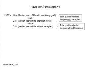
The LYFT score for each candidate is calculated using the estimated median survival times (measured in years) without a transplant, based on candidate characteristics and with a transplant for each recipient (with and without a functioning graft), based on recipient and donor characteristics. To account for differences in the quality of life with a functioning graft compared with life on dialysis, each year on dialysis is adjusted by a factor of 0.8, based on a synthesis of assessments in the published literature (4, 5), while each year with a functioning graft is given a value of 1.0. The resulting formula used to calculate LYFT is shown in Figure VIII-1.

Click for larger image   Click to view slides for entire chapter

MEASURING TYPICAL LIFETIMES

Several options were considered to estimate the typical lifetimes expected for a group of candidates with a particular set of characteristics. These options included “expected lifetime” (area under the survival curve), “truncated expected lifetime” (area under the survival curve limited to a specified interval, such as up to 10 years), and the “median lifetime,” often referred to as the half-life (i.e., the time at which half of the population has died). Each method provides a measure of the typical life span of patients or grafts bearing the specific characteristics of the candidate, recipient, or graft for whom the life span is being estimated.

Typical lifetimes vary substantially among candidates and recipients. They can be as short as 1.4 years on dialysis alone and 4.2 years Post Transplant for older or less healthy patients. For other groups, especially younger, healthier patients, more than 50% of patients were still alive 15 years Post Transplant.

One of the challenges was to identify an appropriate metric of expected lifetime that would yield accurate and meaningful estimates at the extremes of age and health. It is important to recognize, since the LYFT calculation is the difference between expected Post Transplant and waiting list survivals, that all else being equal, LYFT scores will be highest not only for candidates with relatively longer expected Post Transplant survival but also for candidates with relatively shorter waiting list survival (medical urgency). Calculation of LYFT scores among subpopulations of candidates are elaborated below in the section, “LYFT Scores versus Candidate Demographics.”

Life years as calculated from the area under the survival curve for a population was initially considered for calculating LYFT. Area under the survival curve estimates the average lifetime of that population. However, the area under the survival curve could not be calculated directly with available data for those populations for which a substantial fraction were still alive at the end of follow-up (15 years). Furthermore, the area under the survival curve, beyond the end of follow-up, cannot be estimated using standard Cox regression techniques. Therefore, alternative methods for estimating lifetimes were investigated.

The OPTNKC also considered calculations of lifetimes truncated at a fixed number of years, starting with 10 years, based on the area under the survival curve up to the prescribed number of years. Although this area can be calculated with the available data, the resulting metrics exclude from the survival calculation a portion of the LYFT that many, especially younger and healthier, candidates could expect to achieve. Potentially short-lived recipients tend to gain their LYFT soon after transplant (within 5 to 10 years), while longer-lived recipients are more likely to realize their LYFT several years later (15 to 25 years after transplant). Thus, truncation even at 10 or 20 years would arbitrarily exclude from survival calculations much of the LYFT that is attained by long-lived candidates. This concept is illustrated in Figures VIII-2 and VIII-3. In Figure VIII-2, measurement of survival is truncated at five years for a hypothetical population of patients; the difference between the area under the resultant recipient and candidate survival curves is larger for patients transplanted at the age of 50 years than it is for those transplanted at 20 years. In Figure VIII-3, greater than 30 years of Post Transplant survival is hypothetically captured. In contrast to Figure VIII-2, the difference between the area under the resultant recipient and candidate survival curves is now larger for 20 year-old patients than it is for those 50 years old. In addition, the OPTNKC is interested in minimizing the transplantation of kidneys with the potential for long Post Transplant survival into recipients at high risk for early death with a functioning transplant. Thus, it was important to use a metric that was appropriate for longer-lived candidates.

Click for larger image   Click to view slides for entire chapter

Click for larger image   Click to view slides for entire chapter

In contrast, the median lifetime can be estimated for the majority of candidates without projection of the survival curve beyond 15 years. The median lifetime was less than 15 years and could thus be estimated directly from existing data for 99% of lifetimes without transplant and for 72% of Post Transplant lifetimes with an average non-expanded criteria donor (non-ECD) kidney. (Note: By the OPTN definition, ECD kidneys are defined as having a risk of graft failure (1.7 times that of ideal donors. ECDs include any donor (60 years and donors 50-59 years with at least two of the following: terminal creatinine >1.5 mg/dl, history of hypertension, or death by cerebrovascular accident.) For the remainder of candidates and recipients, extrapolation methods were used to estimate the median lifetime (see “Long-Term Survival and Extrapolation” below). The median estimated lifetimes were much more consistent for longer (over 15 years) lifetimes with alternative extrapolation methods than were those calculated using the area under the survival curve.

MODELING

Separate models were estimated for short-term (years 0 - <4) and long-term (years 4-15) survival with transplant, survival without transplant, and graft survival, for a total of six models in all. The short-term models predicted survival out to four years, while the long-term models estimated survival to 15 years, conditional on surviving the first four years. The four-year cut point was chosen because it best fit the shapes of the survival curves and because it is well beyond the period of elevated death rates that persisted for longer than one year following transplant for some patient groups. The same four-year cutoff also allowed the waiting list and Post Transplant survival models to accommodate covariates with potentially non-proportional associations with short-term versus long-term death rates.

Survival without transplant was estimated based on death rates among patients who had been listed for transplantation. The data used to estimate survival without a transplant includes pretransplant data for those candidates who received a transplant, data for candidates who were wait-listed but not yet transplanted, data up until the time of death for candidates who died on the waiting list, and follow-up data for candidates who were removed from the waiting list for reasons other than death or transplantation. Similarly, survival with transplant includes survival time after graft failure, censored at re-transplantation. Graft survival was calculated as the time to death or graft failure, whichever occurred sooner. Life span after graft failure was calculated as the difference between life span following transplant and the life span of the functioning graft. Covariate selection was carried out separately for each of the six models. Short-term and long-term survival models were not required to contain the same variables, as described in the section below, “Covariates Used to Estimate Short-Term and Long-Term Survival.”

DATA

Descriptive Statistics

Calculation of LYFT depends on models used to estimate survival both with and without a kidney transplant. Survival without a kidney transplant is estimated using past waiting list data; survival with a kidney transplant is estimated using past data on kidney recipients.

Models used to estimate survival without a transplant are based on candidates active on the waiting list on January 1 of each of 1988, 1990, 1994, 1998, and 2002. These samples were aggregated to include both long-term survival (from older cohorts) and recent survival (from recent cohorts). Only adult candidates for deceased donor kidneys (even if they eventually received a living donor kidney) and recipients of deceased donor kidneys were included. Recipient survival was censored at the time of transplant for those candidates who received a subsequent kidney, but this re-transplantation, if preemptive, counted as a graft failure in graft survival models.

Models of both patient and graft survival after transplant were based on all non-ECD kidney and SPK transplants from 1987 to 2006. Simultaneous kidney with extra-renal organ transplants, with the exception of SPK transplants, were excluded.

The resulting sample sizes for the different models and periods are shown in Table VIII-1. Table VIII-2 displays descriptive statistics of the data used to build the models for estimating the median waiting list and Post Transplant survival times, and, as an example, for adult candidates active on a specific sample offer date (January 1, 2004). Using the cross-section of active candidates on a given date provided general information on the demographics of typical candidates who might be active at the time of an organ offer. This cross-section is used below in the section, “LYFT Scores Versus Candidate Demographics,” to illustrate differences in LYFT scores among an average group of candidates who might be available for transplant on a given date.

Table VIII-1. Sample Size

Table VIII-2: Mean (SD) of Variables Used in LYFT Calculations

Variables Used or Investigated for Use in the LYFT Calculation

There are separate models for the three types of survival.

WL (Waiting List): Candidate survival without transplant is calculated from a given calendar date, rather than the individual listing dates. The cross-sectional nature of the sample selection allows the survival patterns used in the LYFT calculation to mimic those seen in the prevalent waiting list population upon which allocation is based and not the incident waiting list, which contributes to but does not replicate the candidate list at any particular moment in time (6).

PT (Post Transplant): Recipient survival with a transplant. This includes all post-operative mortality, but survival time is censored on retransplant.

GS (Graft Survival): Graft survival after a transplant. For kidney-pancreas recipients, this is the survival of the kidney, not the pancreas graft.

Short- and long-term survival for each model was estimated separately. Short-term survival during the 0-4 year period after a given calendar date, mimicking the survival of non-recipients after an offer (WL) or of recipients after transplant (PT or GS), is indicated by “0 - <4” in the column header of Tables VIII-3 and VIII-4, and long term survival is indicated by “4-15.” Hazard ratios in bold italics show that the variable was significant (p<0.05) in the specific model listed in the column header.

Table VIII-3: Hazard Ratios of Variables Used in LYFT Calculation

Table VIII-4: Additional Variables Considered for LYFT Calculation: Hazard Ratio (Index of Concordance [IoC])

MODEL DIAGNOSTICS

In this section, we describe the methods used to evaluate the survival models upon which the LYFT calculations are based, beginning with a summary measure of a model's predictive capacity and followed by an assessment of its underlying assumptions.

Predictive Capability of the Models:

The index of concordance (IOC) is an overall measure of goodness of fit that gauges a model’s ability to successfully rank patient survival. The IOC is computed as the proportion of patient pairs for which the model correctly predicts ordering of the survival times. The IOC ranges from 0.5 to 1.0, with 0.5 indicating that the model is unable to rank candidates and with 1.0 indicating that the model ranks candidates perfectly according to their survival. The index of concordance was calculated by using a random half of the available data to create the model and a random sub-sample of the other half of the available data to test the model’s predictive capability. The IOC is provided for each model component in the first row of Table VIII-3.

Evaluating Proportional Hazards

Based on statistical diagnostic tests, we identified factors which appeared to have non-proportional hazards effects. The following discussion lists the covariates for which the proportional hazards assumption did not hold and explains the procedures used to account for this non-proportionality.

Verifying Proportional Hazards in LYFT Covariates. Statistical tests were performed to determine whether there were any significant changes in the variable effects over time within each period (0 - <4 years vs. 4-15 years on the waiting list or after transplant). Every main effect covariate used in the LYFT calculation was tested in each of the models to determine if the proportional hazard assumption held during all periods. Each test was done in a separate model, where the variable being tested was included both as a baseline characteristic and as a time-dependent characteristic interacting multiplicatively with linear time.

To speed processing, a 1/10th random sample of candidates and recipients was used. This left 2,608 candidates with 685 events for the smallest data set; namely the 4-15 year period for survival without transplant. The other three models had between 1,700 and 2,400 events.

The covariates indicating diabetes and whether the recipient received an SPK transplant were known to be non-proportional before this testing. As a consequence, these tests were performed on models in which these factors were stratified into three groups: non-diabetic recipients, diabetic kidney recipients, and diabetic kidney-pancreas recipients.

Of the 70 tests of time-dependent covariates conducted, four were statistically significant with p values below 0.05. The four factors were: zero HLA mismatch (MM) (Post Transplant model for the 4-15 year period, parameter=-0.13, p=0.05), cohort year (without-transplant model for the 4-15 year period, parameter=0.015, p=0.04), preemptive listing and still not on dialysis at offer (without-transplant model for the 4-15 year period, parameter=-0.081, p=0.04), log of donor weight (Post Transplant model for the 4-15 year period, parameter=0.17, p=0.01). These factors will be investigated further but were left as proportional hazards in this iteration of the LYFT modeling. This approach will account for these factors on the basis of their average effect during the follow-up interval.

The proportional hazards assumption seems to hold overall in each of the models used, and no time-dependent factors have been included in the LYFT calculations.

Kidney Alone versus Simultaneous Kidney-Pancreas, Diabetic versus Non-Diabetic. The waiting list models for kidney non-diabetic, kidney diabetic, and kidney-pancreas survival showed that the death rates for these three groups were close to proportional throughout 10 years of follow-up and that the kidney non-diabetic and kidney diabetic groups were nearly proportional for years 10-17. The models for survival with transplant for kidney non-diabetic, kidney diabetic, and kidney-pancreas survival showed that the death rates for these three groups were not proportional.

All Cox models of survival after transplant used to estimate LYFT are stratified into three groups: non-diabetic kidney transplants, diabetic kidney transplants, and kidney-pancreas transplants with different regression coefficients used in each group, when there was evidence that the coefficients differed by group. Unlike the models of survival after transplant, the model of candidate survival without transplant did not stratify by diabetes status or transplant type. This allowed the use of the proportional hazards assumption to complete the kidney-pancreas survival curve through 15 years, as there were insufficient kidney-pancreas candidates with survival beyond 10 years to define a separate survival curve. In other words, the hazards for kidney-pancreas candidates were assumed to continue to be proportional to those of kidney candidates after the period during which the hazard for kidney-pancreas candidates could be independently estimated. This assumption meant kidney-pancreas candidate survival without transplant could be estimated based on functions of kidney candidate survival without transplant.

Covariates Used to Estimate Short-Term and Long-Term Survival. Some factors used in the LYFT models that were significant predictors of short-term (0 - <4 year) survival were not predictive of long-term survival and were thus not included in the long-term (4-15 year) models (Table VIII-5). The use of separate models for short-term and long-term survival also allowed the effects of covariates to differ for short- versus long-term survival, thereby allowing for possible non-proportional effects.

Table VIII-5: Factors Not Significantly Predictive of Survival 4-15 Years After Offer or Transplant

Testing Interactions

Both clinical judgment and statistical analysis were used to determine the interaction terms used in the LYFT calculations. Table VIII-6 shows the interaction terms used.

Table VIII-6: Interaction Terms Used in LYFT Calculations

Testing Linearity of Effect

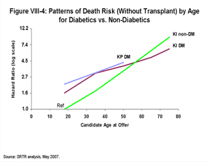
Candidate Age at Offer or Transplant. Candidate age at offer or transplant was found to be a nearly linear effect, as shown in Figure VIII-4, which displays the log-hazard ratio (i.e., the log of the relative death rate, compared with that of 18 year-old non-diabetics) versus candidate age, where the slope for candidate age is allowed to change at specified ages according to the data.

Click for larger image   Click to view slides for entire chapter

After reviewing the results shown in Figure VIII-4 and similar results for transplant recipients, the effect of age on death rates in each of the regression models was included as a continuous, linear age predicting the log hazard ratio. Interaction terms between age and diabetes (DM) for kidney-alone (KI nonDM and KI DM) and kidney-pancreas (KP DM) were included in the without-transplant model to account for differences in the effects of age between patients with and without diabetes. Interaction terms between age and diabetes were also included in the with-transplant model.

All Other Covariates. Several factors were found to have non-linear effects on the outcome in at least one of the models. For certain terms (e.g., time on dialysis, donor weight) log transformations resulted in a better fit according to likelihood ratio tests. For panel reactive antibody (PRA) values, categorical variables for different levels seemed the best approach to the OPTNKC, since the existing national kidney allocation policy treats highly sensitized (PRA 80% or higher) candidates differently. Other non-linear effects were modeled using splines. Instead of a single straight line, the spline approach models the effect as a series of connected straight lines, where the slope was allowed to change as dictated by the data (as shown in Figure VIII-4).

If a non-linear effect was found for one model, it was kept for all models that included that covariate. Table VIII-7 lists the factors where non-linear terms were used.

Table VIII-7: Non-Linear Parameterizations of Continuous Variables Used in LYFT

LONG-TERM SURVIVAL AND EXTRAPOLATION

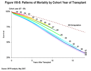
Long-Term Survival Based on Older Data

Older data were used to obtain the long-term survival estimates, but survival levels were adjusted to reflect recent experience. The survival curves for each cohort year shown in Figure VIII-5 illustrate this process. The shape of the survival curve for the year 2006 non-diabetic kidney transplant recipients (topmost) is solid for one year, where actual data are available, and dotted afterward, indicating the extrapolation period. The extrapolation of this curve is based on older experience, as shown by the solid lines for previous years; but, the fact that 2006 recipients have had better survival than their counterparts in previous cohorts during the comparable period after transplant is also accounted for. The baseline survival curve in each LYFT calculation is estimated out to year 15 using a Cox model with indicator variables for each cohort year with adjustment, in a manner similar to the example adjustment for the year 2006 shown in Figure VIII-5.

Click for larger image   Click to view slides for entire chapter

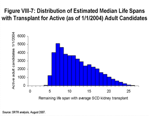
Amount of Extrapolation Required. When calculating the median remaining life span for candidates active on the waiting list on a given date, (e.g., January 1, 2004), only about 1% require extrapolation beyond the 15-year survival curve described in the prior section. Transplant recipients have longer life spans, and about 28% of the candidates active on the list on January 1, 2004 would require extrapolation to determine their median life span if they were to receive a non-ECD kidney.

For purposes of illustration, the following histograms (Figures VIII-6 and VIII-7) show the distributions of remaining life spans for adult candidates active on the kidney (or kidney-pancreas) waiting list on January 1, 2004, if they never received a transplant (Figure VIII-6) and if they all received a non-ECD kidney (or kidney-pancreas) from a donor with the mode characteristics of actual donors from the 2003 deceased donor pool (Figure VIII-7).

Click for larger image   Click to view slides for entire chapter

Click for larger image   Click to view slides for entire chapter

Details of Extrapolation Beyond 15 Years of Median Survival. While the initial hazard after transplant is elevated, the log of the long-term (more than four years) hazard appears to be reasonably well approximated as linear growth over time, suggesting that the growth in death rates can be approximated as exponential growth with time (7). The linear growth in the log hazard over time is also similar (proportional) to that of the general population, as shown by the roughly parallel plots of the death rate per year on the log scale in Figure VIII-8. Upper curves in this figure indicate the death rate per year (starting four years after offer or transplant) for otherwise-average candidates who at age 45 years either remain untransplanted (uppermost line, starting four years after an arbitrary offer), receive a kidney transplant as a diabetic (second highest line), receive a SPK transplant (third highest line), or receive a kidney transplant as a non-diabetic (fourth line). The death rates start four years after offer or transplant for each group in order to emphasize the trend associated with increasing age, rather than the relatively brief postoperative elevation in death rates in the transplant groups. The slopes actually used for extrapolation in the LYFT calculation are detailed in Table VIII-8. The absolute mortality remains lowest for the general population and highest for the waiting list. Post Transplant mortality increases with time in a manner similar to that of the general population, while waiting list mortality, although higher overall, may increase more slowly with time.

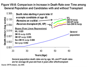Click for larger image   Click to view slides for entire chapter

Table VIII-8: Slope of Long-Term Log-Hazard Over Time

LYFT SCORES VERSUS CANDIDATE DEMOGRAPHICS

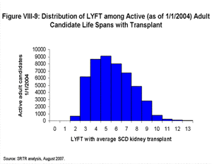
The histogram in Figure VIII-9 shows the overall distribution of LYFT scores for adult kidney and kidney-pancreas candidates active on the waiting list on January 1, 2004 had they each received an average non-ECD kidney.

Click for larger image   Click to view slides for entire chapter

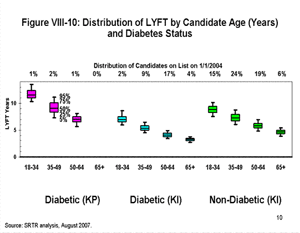
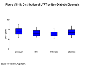
Box Plots of Distribution of LYFT by Demographic

Each box plot (Figures VIII-10, VIII-11, VIII-12, VIII-13, VIII-14, VIII-15 and VIII-16) shows the distribution of LYFT scores among kidney and kidney-pancreas candidates active on the waiting list on January 1, 2004 using the box for the interquartile range (25th through 75th percentile) and whiskers for the 5th and 95th percentiles. The horizontal line within the box is the median LYFT score for the population depicted. The LYFT scores are calculated based on a kidney or kidney-pancreas donor with the average characteristics of a non-ECD donor; averages apply to both donor-alone factors such as donor age (32 years) and to shared donor/recipient factors such as level of HLA mismatch. The distribution of candidate variables (e.g., body mass index [BMI], diagnosis, time since starting dialysis, etc.) reflects those actually seen in the candidate and recipient populations in 2003, the year represented in the model. The distribution of LYFT scores within the box and whisker plots reflects the effects of these variables among the represented patients.

Click for larger image   Click to view slides for entire chapter

Click for larger image   Click to view slides for entire chapter

Click for larger image   Click to view slides for entire chapter

Click for larger image   Click to view slides for entire chapter

Click for larger image   Click to view slides for entire chapter

Click for larger image   Click to view slides for entire chapter

Click for larger image   Click to view slides for entire chapter

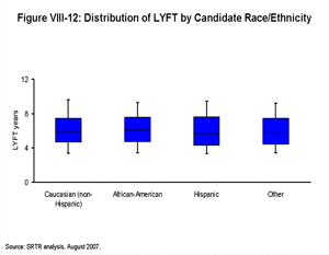
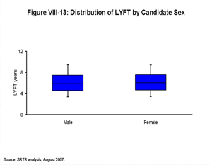
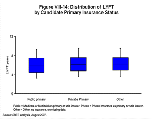
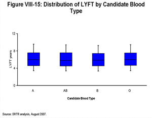
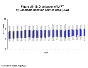
Figure VIII-10 demonstrates the range and median of LYFT scores for all candidates by age and diagnosis categories. The percentages at the top of the figure represent the proportion of these individuals in the candidate population. LYFT scores in general are higher among younger candidates and for diabetic candidates awaiting an SPK transplant; they are lower for older candidates and for diabetic candidates listed for kidney transplantation alone. The distributions of the LYFT scores are very similar across categories of other patient subpopulations (diagnosis among non-diabetics, race/ethnicity, sex, insurance status, blood type, and DSA) as shown in Figures VIII-11, VIII-12, VIII-13, VIII-14, VIII-15 and VIII-16.

Independent Effects on LYFT (All Else Equal)

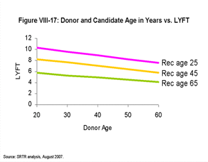
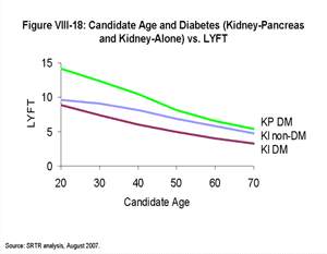
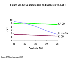
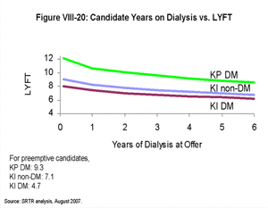
Figures VIII-17, VIII-18, VIII-19, and VIII-20 demonstrate the estimated LYFT for a hypothetical group of almost-identical candidates who only differ by the factor noted. In contrast to the box plots (Figures VIII-10, VIII-11, VIII-12, VIII-13, VIII-14, VIII-15 and VIII-16) that display the range of LYFT scores among actual candidate groups (which tend to differ by more than one factor), these graphics show the estimated relative effects of certain example factors on LYFT. The purpose of Figures VIII-17, VIII-18, VIII-19, and VIII-20 is to show the effect of single example factors on LYFT with all else held equal, not to depict ranges of LYFT scores for actual candidate groups.

Click for larger image   Click to view slides for entire chapter

Click for larger image   Click to view slides for entire chapter

Click for larger image   Click to view slides for entire chapter

Click for larger image   Click to view slides for entire chapter

DISCUSSION

LYFT, estimated using regression models based on candidate and donor data, provides information about the quality-adjusted extra years of life that a given transplant could be expected to provide for a given patient. This could be a valuable tool in allocation of deceased-donor kidneys, evaluation of kidney allocation methods, and patient counseling. Prioritizing the candidates with the higher LYFT scores for each kidney that becomes available could increase the average extra years of life of a transplant by about one year compared with the current system; accordingly, a year’s worth of kidneys allocated in this way could provide in aggregate around 10,000 extra years of life (8).

The concept of LYFT is useful both for designing an effective organ allocation system and for advising candidates of treatment options.

In organ allocation, LYFT could be calculated when a kidney becomes available, based on the donor’s characteristics and those of the candidates active on the waiting list. Prioritizing offers to candidates with large LYFT scores would lead to more years of life among candidates and recipients, in total.

When informing a single candidate of personal treatment options, LYFT could be calculated using the characteristics of that candidate for a range of several possible donor kidneys that might become available in the future (e.g., ECD, non-ECD, and living donor). This information, along with candidate health status and the likelihood of receiving various types of kidneys, could be used, for example, to make informed decisions about whether to rule out offers of certain types of donor kidneys for a specific candidate.

A kidney allocation system incorporating LYFT could be modified to incorporate goals other than that of increasing the total candidate life span. For example, the LYFT scores shown in this article, reflecting the direction chosen by the OPTNKC, are modified by a conversion factor for quality of life. Years with a functioning transplant are given a weight of one, whereas waiting list years and years after graft failure are given a weight of 0.8. Calculation of the expected years of graft survival allows the components of LYFT to be weighted according to these differences in quality of life. Other modifications to LYFT could include a weighting system that would discount years in the future compared with years occurring sooner or could add more emphasis to waiting list urgency. The models used to calculate LYFT are expected to be updated as additional data become available and refined as needed. Among the alternatives under consideration are the inclusion of ECD kidneys and the exclusion of SPK recipients in the models used to estimate LYFT. In addition, other elements could be blended into the kidney allocation algorithm that would give allocation priority based upon consideration other than expected LYFT. Such factors as waiting time, PRA, and prior donation serve other legitimate allocation priorities. Changes in LYFT resulting from modification of allocation rules can be used as a metric to gauge the consequences of these rules on Post Transplant patient survival.

SUMMARY

LYFT, estimated using regression models based on candidate and donor data, provides information about the quality-adjusted survival benefit that a given transplant could provide a given patient. This measure can be estimated by Cox proportional hazards regression models without violating the assumptions inherent in using these models; it can incorporate a factor to account for the difference in quality of life with and without a functioning graft; LYFT can be estimated without extrapolating beyond available data for the majority of the candidates for a particular kidney; and it can be estimated using reasonable extrapolation methods for the remaining candidates. This could be a valuable tool in the allocation of deceased-donor kidneys, evaluation of kidney allocation methods, and patient counseling. By prioritizing the candidates with the higher LYFT scores for each kidney that becomes available, each year’s worth of kidneys could provide over 10,000 extra years of life beyond the benefit provided by the same kidneys under the current system (7).

REFERENCES

1. McCullough KP, Leichtman AB, Port FK, Wolfe RA. Trends in kidney recipient age and survival benefit due to transplant by year [abstract].” Am J Transplant 2007; 7: 231.

2. Wolfe RA, Ashby VB, Milford EL, et al. Comparison of mortality in all patients on dialysis, patients on dialysis awaiting transplantation, and recipients of a first cadaveric transplant. N Engl J Med 1999; 341: 1725-1730.

3. Marubini E, Valsecchi MG. 1995. Analysing Survival Data from Clinical Trials and Observational Studies. John Wiley & Sons, Ltd. p. 171.

4. Andreas L, Keown P, Pus N, Krueger H, Ferguson B, Wong C, Muirhead N. A study of the quality of life and low cost-utility of renal transplantation. Kidney Int 1996; 50: 235-242.

5. Hornberger JC, Best JH, Garrison LP. Cost-effectiveness of repeat medical procedures: Kidney transplantation as an example. Med Decis Making 1997; 17: 363-372.

6. Wolfe, RA. “Avoiding statistical bias in predicting the life years from transplant (LYFT)” p. 18. SRTR Working Paper. Available at https://ustransplant.org/kars.aspx. Accessed December 14, 2007.

7. Wolfe, RA “Extrapolation methods: approximating the median survival time beyond the duration of follow-up based on geometric and linear growth in death rates” SRTR Working Paper. Available at https://ustransplant.org/kars.aspx. Accessed December 14, 2007.

8. Wolfe RA, McCullough KP, Rodgers A, Leichtman AB. A modification to kidney transplant allocation to save more patient years of life [abstract].” Am J Transplant 2007;7(2): 230.